Fermat’s Last Theorem
As a pure mathematician Newton reached his climax in the invention of the calculus, an invention also made independently by Leibniz. But do you know that, Fermat conceived and applied the leading idea of the differential calculus thirteen years before Newton was born and seventeen before Leibniz was born.
Today we are going delve into Fermat’s last work, whose proof took three and a half centuries to hail again after Fermat. Its nothing but Fermat’s Last Theorem.
We will start to take our steps towards the brilliance of this theorem by learning a bit about the Pythagorean Triples.Pythagorean triples have been known since ancient times. The oldest known record comes from Plimpton 322, a Babylonian clay tablet from about 1800 BC, written in a sexagesimal number system. A Pythagorean triple consists of three positive integers a, b, and c, such that a2 + b2 = c2. The equation a2 + b2 = c2 is a Diophantine equation.
(3, 4, 5) (5, 12, 13) (8, 15, 17) (7, 24, 25) (20, 21, 29) (12, 35, 37) (9, 40, 41) (28, 45, 53) (11, 60, 61) (16, 63, 65) (33, 56, 65) (48, 55, 73) (13, 84, 85) (36, 77, 85) (39, 80, 89) (65, 72, 97) 16 primitive Pythagorean triples with c ≤ 100 The Theorem
The proposition was first conjectured by Pierre de Fermat around 1637 in the margin of a copy of Arithmetica; Fermat added that he had a proof that was too large to fit in the margin.

Fermat’s Last Theorem states that no three positive integers a, b, and c satisfy the equation an + bn = cn for any integer value of n greater than 2.
After 358 years of effort by mathematicians, the first successful proof was released in 1994 by Andrew Wiles, and formally published in 1995; it was described as a “stunning advance” in the citation for Wiles’s Abel Prize award in 2016. Wiles’s proof also proved much of the modularity theorem and opened up entire new approaches to numerous other problems and mathematically powerful modularity lifting techniques.
The Big Picture
Wiles’ three groundbreaking lectures, in June 1993, at the Isaac Newton Institute in Cambridge, UK were inspirational and shaped mathematics in its own way.
Theorem. Every semistable elliptic curve over Q is modular.
The strategy that ultimately led to a successful proof of Fermat’s Last Theorem was the connection with elliptic curves which arose from the “astounding” Taniyama–Shimura–Weil conjecture, proposed around 1955 which many mathematicians believed would be near to impossible to prove, and was linked in the 1980s by Gerhard Frey, Jean-Pierre Serre and Ken Ribet to Fermat’s equation. By accomplishing a partial proof of this conjecture in 1994, Andrew Wiles ultimately succeeded in proving Fermat’s Last Theorem, as well as leading the way to a full proof by others of what is now the modularity theorem.
The Taniyama-Shimura conjecture
The Taniyama-Shimura conjecture, since its proof now sometimes known as the modularity theorem, is very general and important conjecture (and now theorem) connecting topology and number theory which arose from several problems proposed by Taniyama in a 1955 international mathematics symposium.
The Shimura-Taniyama-Weil conjecture relates elliptic curves (cubic equations in two variables of the form y2 = x3 + ax + b, where a and b are rational numbers) and modular forms, objects (to be defined below) arising as part of an ostensibly different circle of ideas. An elliptic curve E can be made into an abelian group in a natural way after adjoining to it an extra “solution at infinity” that plays the role of the identity element. This is what makes elliptic curves worthy of special study, for they alone, among all projective curves (equations in two variables, compactified by the adjunction of suitable points at infinity) are endowed with such a natural group law. If one views solutions geometrically as points in the (x, y)-plane, the group operation consists in connecting two points on the curve by a straight line, finding the third point of intersection of the line with the curve and reflecting the resulting point about the x-axis.
The entire proof is not possible to provide through this post but a link will suffice it.
Courtesies- https://www.wikipedia.org/, THE PROOF OF FERMAT’S LAST
THEOREM by Nigel Boston University of Wisconsin – Madison.THE SOUL THEOREM

We think mathematics to be a subject too coarse to have a connection to any spirit, let alone to have its own. But Mathematicians are probably the only people to have named a theorem ‘THE SOUL THEOREM’. The soul theorem is a theorem of Riemannian geometry that largely reduces the study of complete manifolds of non-negative sectional curvature to that of the compact case. Every compact manifold is its own soul. In 1972, Cheeger and Gromoll proved the theorem by the generalization of a 1969 result of Gromoll and Wolfgang Meyer. The related soul conjecture was formulated by Gromoll and Cheeger in 1972 and proved by Grigori Perelman in 1994 with an astonishingly concise proof.
The theorem states,
If (M, g) is a complete connected Riemannian manifold with sectional curvature K ≥ 0, then there exists a compact totally convex, totally geodesic submanifold S whose normal bundle is diffeomorphic to M. (Note that the sectional curvature must be non-negative everywhere, but it does not have to be constant.) Such a submanifold S is called a soul of (M, g).
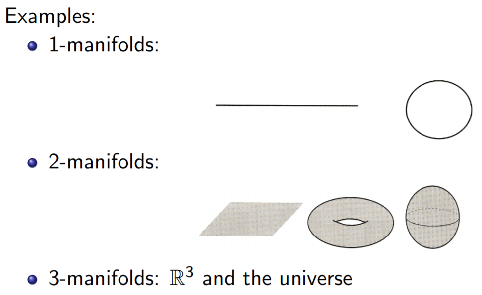
Manifolds in mathematics are topological spaces that resembles Euclidean spaces near each point locally. An n-dimensional manifold is precisely a topological space with the property that each point has a neighborhood that is homeomorphic to the Euclidean space of dimension n. In topology, two objects have the same shape if one can be deformed into the other without cutting or gluing. Objects with the same shape are called homeomorphic.

JUST TRY TO IMAGINE A 4 – MANIFOLD. SOUL CONJECTURE
The Cheeger and Gromoll’s soul conjecture states,
Suppose (M, g) is complete, connected and non-compact with sectional curvature K ≥ 0, and there exists a point in M where the sectional curvature (in all sectional directions) is strictly positive. Then the soul of M is a point; equivalently M is diffeomorphic to Rn.
Grigori Perelman established that in the general case K ≥ 0, Sharafutdinov’s retraction P : M → S is a submersion and hence proved the soul conjecture.
In this note we consider complete noncompact Riemannian manifolds M of nonnegative sectional curvature. The structure of such manifolds was discovered by Cheeger and Gromoll : M contains a (not necessarily unique) totally convex and totally geodesic submanifold S without boundary, 0 < dimS < dimM, such that M is diffeomorphic to the total space of the normal bundle of S in M . (S is called a soul of M.) In particular, if S is a single point, then M is diffeomorphic to a Euclidean space. This is the case if all sectional curvatures of M are positive, according to an earlier result of Gromoll and Meyer. Cheeger and Gromoll conjectured that the same conclusion can be obtained under the weaker assumption that M contains a point where all sectional curvatures are positive. A contrapositive version of this conjecture expresses certain rigidity of manifolds with souls of positive dimension. It was verified in the cases dim S = 1 and codimS = 1, and by Marenich, Walschap, and Strake in the case codimS = 2.
EXAMPLE,
As a very simple example, take M to be Euclidean space Rn. The sectional curvature is 0 everywhere, and any point of M can serve as a soul of M. Now take the paraboloid M = {(x, y, z) : z = x2 + y2}, with the metric g being the ordinary Euclidean distance coming from the embedding of the paraboloid in Euclidean space R3. Here the sectional curvature is positive everywhere, though not constant. The origin (0, 0, 0) is a soul of M. Not every point x of M is a soul of M, since there may be geodesic loops based at x, in which case
 wouldn’t be totally convex.
Citation
Perelman, G. Proof of the soul conjecture of Cheeger and Gromoll. J. Differential Geom. 40 (1994), no. 1, 209–212. doi:10.4310/jdg/1214455292.
Processing…Success! You're on the list.Whoops! There was an error and we couldn't process your subscription. Please reload the page and try again.
Newton’s Three Body Problem
THE GALACTIC CHAOS
The classical three-body problem arose in an attempt to understand the effect of the Sun on the Moon’s Keplerian orbit around the Earth. It has attracted the attention of some of the best physicists and mathematicians and led to the discovery of ‘chaos’. We survey the three-body problem in its historical context and use it to introduce several ideas and techniques that have been developed to understand classical mechanical systems.
The study of the three-body problem led to the discovery of the planet Neptune, it explains the location and stability of the Trojan asteroids and has furthered our understanding of the stability of the solar system. Quantum mechanical variants of the three-body problem are relevant to the helium atom and water molecule.

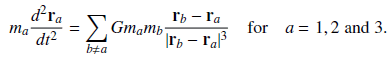
We consider the problem of three point masses (ma with position vectors ra for a = 1, 2, 3) moving under their mutual gravitational attraction. This system has 9 degrees of freedom, whose dynamics is determined by 9 coupled second order nonlinear ODEs:

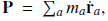
As before, the three components of momentum,

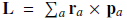
three components of angular momentum,

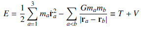
and energy,

Wolfgang Pauli (1926) derived the quantum mechanical spectrum of the Hydrogen atom using the relation between E, L2 and A2 before the development of the Schrodinger equation. Indeed, if we postulate circular Bohr orbits which have zero eccentricity (A = 0) and quantized angular momentum L^2 = n^2(h/2pi)^2, then En = − (mα^2)/ (2(h/2pi)^2n^2) where α = e^2/4πϵ0 is the electromagnetic analogue of Gm1m2.

General solutions
There is no general analytical solution to the three-body problem given by simple algebraic expressions and integrals. Moreover, the motion of three bodies is generally non-repeating, except in special cases.
On the other hand, in 1912 the Finnish mathematician Karl Fritiof Sundman proved that there exists a series solution in powers of t1/3 for the 3-body problem. This series converges for all real t, except for initial conditions corresponding to zero angular momentum. (In practice the latter restriction is insignificant since such initial conditions are rare, having Lebesgue measure zero.)
An important issue in proving this result is the fact that the radius of convergence for this series is determined by the distance to the nearest singularity. Therefore, it is necessary to study the possible singularities of the 3-body problems. As it will be briefly discussed below, the only singularities in the 3-body problem are binary collisions (collisions between two particles at an instant) and triple collisions (collisions between three particles at an instant).
Collisions, whether binary or triple (in fact, any number), are somewhat improbable, since it has been shown that they correspond to a set of initial conditions of measure zero. However, there is no criterion known to be put on the initial state in order to avoid collisions for the corresponding solution. So Sundman’s strategy consisted of the following steps:
- Using an appropriate change of variables to continue analyzing the solution beyond the binary collision, in a process known as regularization.
- Proving that triple collisions only occur when the angular momentum L vanishes. By restricting the initial data to L ≠ 0, he removed all real singularities from the transformed equations for the 3-body problem.
- Showing that if L ≠ 0, then not only can there be no triple collision, but the system is strictly bounded away from a triple collision. This implies, by using Cauchy’s existence theorem for differential equations, that there are no complex singularities in a strip (depending on the value of L) in the complex plane centered around the real axis (shades of Kovalevskaya).
- Find a conformal transformation that maps this strip into the unit disc. For example, if s = t1/3 (the new variable after the regularization) and if |ln s| ≤ β, then this map is given by
Unfortunately, the corresponding series converges very slowly. That is, obtaining a value of meaningful precision requires so many terms that this solution is of little practical use. Indeed, in 1930, David Beloriszky calculated that if Sundman’s series were to be used for astronomical observations, then the computations would involve at least 108000000 terms.
n-body problem
The three-body problem is a special case of the n-body problem, which describes how n objects will move under one of the physical forces, such as gravity. These problems have a global analytical solution in the form of a convergent power series, as was proven by Karl F. Sundman for n = 3 and by Qiudong Wang for n > 3. However, the Sundman and Wang series converge so slowly that they are useless for practical purposes; therefore, it is currently necessary to approximate solutions by numerical analysis in the form of numerical integration or, for some cases, classical trigonometric series approximations. Atomic systems, e.g. atoms, ions, and molecules, can be treated in terms of the quantum n-body problem. Among classical physical systems, the n-body problem usually refers to a galaxy or to a cluster of galaxies; planetary systems, such as stars, planets, and their satellites, can also be treated as n-body systems. Some applications are conveniently treated by perturbation theory, in which the system is considered as a two-body problem plus additional forces causing deviations from a hypothetical unperturbed two-body trajectory.
The Navier-Stokes Equations
Fluid Dynamics and the Navier-Stokes Equations
The Navier-Stokes equations, developed by Claude-Louis Navier and George Gabriel Stokes in 1822, are equations which can be used to determine the velocity vector field that applies to a fluid, given some initial conditions. They arise from the application of Newton’s second law in combination with a fluid stress (due to viscosity) and a pressure term. For almost all real situations, they result in a system of nonlinear partial differential equations; however, with certain simplifications (such as 1-dimensional motion) they can sometimes be reduced to linear differential equations. Usually, however, they remain nonlinear, which makes them difficult or impossible to solve; this is what causes the turbulence and unpredictability in their results.
Derivation of the Navier-Stokes Equations
The Navier-Stokes equations can be derived from the basic conservation and continuity equations applied to properties of fluids. In order to derive the equations of fluid motion, we must first derive the continuity equation (which dictates conditions under which things are conserved), apply the equation to conservation of mass and momentum, and finally combine the conservation equations with a physical understanding of what a fluid is.Continuity Equation
The basic continuity equation is an equation which describes the change of an intensive property L. An intensive property is something which is independent of the amount of material you have. For instance, temperature would be an intensive property; heat would be the corresponding extensive property. The volume Ω is assumed to be of any form; its bounding surface area is referred to as ∂Ω. The continuity equation derived can later be applied to mass and momentum.General Form of the Navier-Stokes Equation
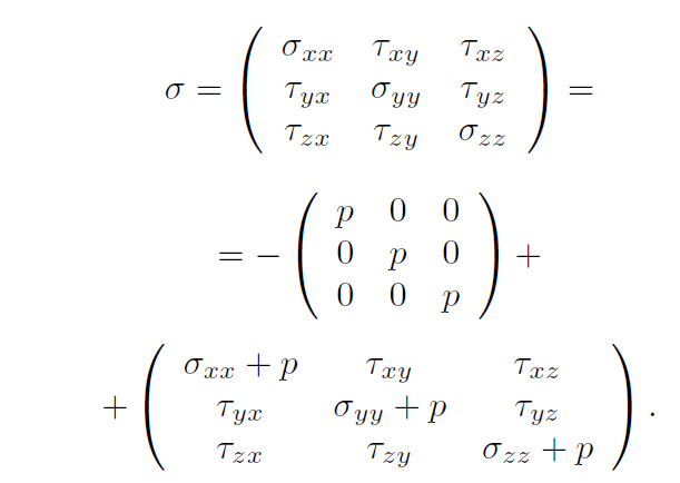
The stress tensor σ denoted above is often divided into two terms of interest in the general form of the Navier-Stokes equation. The two terms are the volumetric stress tensor, which tends to change the volume of the body, and the stress deviator tensor, which tends to deform the body. The volumetric stress tensor represents the force which sets the volume of the body (namely, the pressure forces). The stress deviator tensor represents the forces which determine body deformation and movement, and is composed of the shear stresses on the fluid. Thus, σ is broken down into
Denoting the stress deviator tensor as T, we can make the substitution
σ = −pI + T.Substituting this into the previous equation, we arrive at the most general form of the Navier-Stokes equation:

Although this is the general form of the Navier-Stokes equation, it cannot be applied until it has been more specified. First off, depending on the type of fluid, an expression must be determined for the stress tensor T; secondly, if the fluid is not assumed to be incompressible, an equation of state and an equation dictating conservation of energy are necessary.

Physical Explanation of the Navier-Stokes Equation
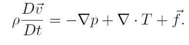
The Navier-Stokes equation makes a surprising amount of intuitive sense given the complexity of what it is modeling. The left hand side of the equation,
is the force on each fluid particle. The equation states that the force is composed of three terms:
• −∇p: A pressure term (also known as the volumetric stress tensor) which prevents motion due to normal stresses. The fluid presses against itself and keeps it from shrinking in volume.
• ∇ · T: A stress term (known as the stress deviator tensor) which causes motion due to horizontal friction and shear stresses. The shear stress causes turbulence and viscous flows – if you drag your hand through a liquid, you will note that the moving liquid also causes nearby liquid to start moving in the same direction. Turbulence is the result of the shear stress.
•~f: The force term which is acting on every single fluid particle. This intuitively explains turbulent flows and some common scenarios. For example, if water is sitting in a cup, the force (gravity) ρg is equal to the pressure term because d/dz (ρgz) = ρg. Thus, since gravity is equivalent to the pressure, the fluid will sit still, which is indeed what we observe when water is sitting in a cup.. Public domain.")
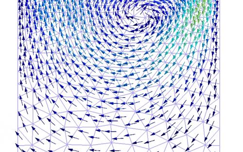
Due to the complex nature of the Navier-Stokes equations, analytical solutions range from difficult to practically impossible, so the most common way to make use of the Navier-Stokes equations is through simulation and approximation. A number of simulation methods exist, and in the next section, we will examine one of the algorithms often used in computer graphics and interactive applications.

Waves follow our boat as we meander across the lake, and turbulent air currents follow our flight in a modern jet. Mathematicians and physicists believe that an explanation for and the prediction of both the breeze and the turbulence can be found through an understanding of solutions to the Navier-Stokes equations. Although these equations were written down in the 19th Century, our understanding of them remains minimal.
The challenge is to make substantial progress toward a mathematical theory which will unlock the secrets hidden in the Navier-Stokes equations.
The Golden Ratio
The ratio, or proportion, determined by Phi (1.618 …) was known to the Greeks as the “dividing a line in the extreme and mean ratio” and to Renaissance artists as the “Divine Proportion” It is also called the Golden Section, Golden Ratio and the Golden Mean.
Just as pi is the ratio of the circumference of a circle to its diameter, phi is simply the ratio of the line segments that result when a line is divided in one very special and unique way.
Divide a line so that:
Definition:
Phi can be defined by taking a stick and breaking it into two portions. If the ratio between these two portions is the same as the ratio between the overall stick and the larger segment, the portions are said to be in the golden ratio. This was first described by the Greek mathematician Euclid, though he called it “the division in extreme and mean ratio,” according to mathematician George Markowsky of the University of Maine.
You can also think of phi as a number that can be squared by adding one to that number itself, according to an explainer from mathematician Ron Knott at the University of Surrey in the U.K. So, phi can be expressed this way: phi^2 = phi + 1
This representation can be rearranged into a quadratic equation with two solutions, (1 + √5)/2 and (1 – √5)/2. The first solution yields the positive irrational number 1.6180339887… (the dots mean the numbers continue forever) and this is generally what’s known as phi. The negative solution is -0.6180339887… (notice how the numbers after the decimal point are the same) and is sometimes known as little phi.
Geometry
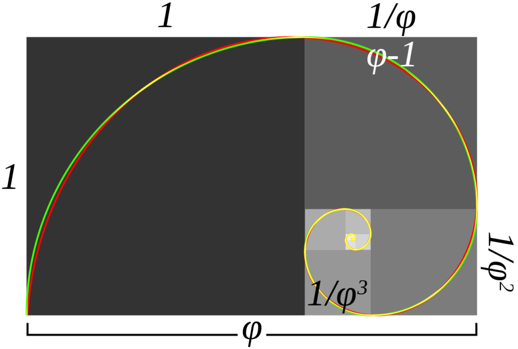
The number φ turns up frequently in geometry, particularly in figures with pentagonal symmetry. The length of a regular pentagon’s diagonal is φ times its side. The vertices of a regular icosahedron are those of three mutually orthogonal golden rectangles.
There is no known general algorithm to arrange a given number of nodes evenly on a sphere, for any of several definitions of even distribution (see, for example, Thomson problem). However, a useful approximation results from dividing the sphere into parallel bands of equal surface area and placing one node in each band at longitudes spaced by a golden section of the circle, i.e. 360°/φ ≅ 222.5°. This method was used to arrange the 1500 mirrors of the student-participatory satellite Starshine-3.

Relationship to Fibonacci sequence
The mathematics of the golden ratio and of the Fibonacci sequence are intimately interconnected. The Fibonacci sequence is:1, 1, 2, 3, 5, 8, 13, 21, 34, 55, 89, 144, 233, 377, 610, 987, …
A closed-form expression for the Fibonacci sequence involves the golden ratio:
The golden ratio is the limit of the ratios of successive terms of the Fibonacci sequence (or any Fibonacci-like sequence), as shown by Kepler:

In other words, if a Fibonacci number is divided by its immediate predecessor in the sequence, the quotient approximates φ; e.g., 987/610 ≈ 1.6180327868852. These approximations are alternately lower and higher than φ, and converge to φ as the Fibonacci numbers increase, and:
More generally:
where above, the ratios of consecutive terms of the Fibonacci sequence, is a case when
Furthermore, the successive powers of φ obey the Fibonacci recurrence:
This identity allows any polynomial in φ to be reduced to a linear expression. For example:
The reduction to a linear expression can be accomplished in one step by using the relationship
where
is the kth Fibonacci number.However, this is no special property of φ, because polynomials in any solution x to a quadratic equation can be reduced in an analogous manner, by applying:
for given coefficients a, b such that x satisfies the equation. Even more generally, any rational function (with rational coefficients) of the root of an irreducible nth-degree polynomial over the rationals can be reduced to a polynomial of degree n ‒ 1. Phrased in terms of field theory, if α is a root of an irreducible nth-degree polynomial, then
, with basis 
Johannes Kepler wrote that “the image of man and woman stems from the divine proportion. In my opinion, the propagation of plants and the progenitive acts of animals are in the same ratio”. The psychologist Adolf Zeising noted that the golden ratio appeared in phyllotaxis and argued from these patterns in nature that the golden ratio was a universal law. Zeising wrote in 1854 of a universal orthogenetic law of “striving for beauty and completeness in the realms of both nature and art”.In 2010, the journal Science reported that the golden ratio is present at the atomic scale in the magnetic resonance of spins in cobalt niobate crystals. However, some have argued that many apparent manifestations of the golden ratio in nature, especially in regard to animal dimensions, are fictitious.
Hilbert’s Grand Hotel Paradox
On a dark desert highway a tired driver passes one more hotel with a “No Vacancy” sign. But this time the hotel looks exceedingly large and so he goes in to see if there might nonetheless be a room for him:
The clerk said, “No problem. Here’s what can be done –
We’ll move those in a room to the next higher one.
That will free up the first room and that’s where you can stay.”The mathematical paradox about infinite sets associated with Hilbert’s name envisages a hotel with a countable infinity of rooms, that is, rooms that can be placed in a one-to-one correspondence with the natural numbers. All rooms in the hotel are occupied. Now suppose that a new guest arrives – will it be possible to find a free room for him or her Surprisingly, the answer is yes. He (or she) may be accommodated in room 1, while the guest in this room is moved to room 2, the guest in room 2 moves to room 3, and so on. Since there is no last room, the newcomer can be accommodated without any of the guests having to leave the hotel. Hilbert’s remarkable hotel can even accommodate a countable infinity of new guests without anyone leaving it. The guests in rooms with the number n only have to change to rooms 2n, which will leave an infinite number of odd-numbered rooms available for the infinite number of new guests. What the parable tells us is that the statement “all rooms are occupied” does not imply that “there is no more space for new guests.” This is strange indeed, although it is not, strictly speaking, a paradox in the logical sense of the term. Yet it is so counter-intuitive that it suggests that countable actual infinities do not belong to the real world we live in.

Hilbert, Cantor, and the infinite.
The discussion of Hilbert’s hotel relates to the old question of whether an actual, as opposed to a potential, infinity is possible. According to Georg Cantor’s theory of transfinite numbers, dating from the 1880s, this is indeed the case, namely in the sense that the concept of the actual infinite is logically consistent and operationally useful [Dauben 1979; Cantor 1962]. But one thing is mathematical consistency, another and more crucial question is whether an actual infinite can be instantiated in the real world as examined by the physicists and astronomers. From Cantor’s standpoint, which can be characterized as essentially Platonic, numbers and other mathematical constructs had a permanent existence and were as real as nay, were more real than – the ephemeral sense impressions on which the existence of physical objects and phenomena are based. From this position it was largely irrelevant whether or not the physical universe contains an infinite number of stars. Contrary to some other contemporary mathematicians, including Leopold Kronecker and Henri Poincaré, Hilbert was greatly impressed by Cantor’s set theory. This he made clear in a semi popular lecture course he gave in Göttingen during the winter semester 1924-1925 and in which he dealt at length with the infinite in mathematics, physics, and astronomy. A few months later he repeated the message in a wide-ranging lecture on the infinite given in Münster on 4 June 1925. The occasion was a session organized by the Westphalian Mathematical Society to celebrate the mathematical work of Karl Weierstrass. Hilbert’s Münster address drew extensively on his previous lecture course, except that it was more technical and omitted many examples. One of them was the infinite hotel. “No one shall expel us from the paradise which Cantor has created for us,” Hilbert famously declared in his Münster address. On the other hand, he did not believe that the actual infinities defined by Cantor had anything to do with the real world.

Möbius Strip
The Möbius Band is an example of one-sided surface in the form of a single closed continuous curve with a twist. A simple Möbius Band can be created by joining the ends of a long, narrow strip of paper after giving it a half, 180°, twist, as in Figure 1. An example of a non-orientable surface, this unique band is named after August Ferdinand Möbius, a German mathematician and astronomer who discovered it in the process of studying polyhedra in September 1858. But history reveals that the true discoverer was Johann Benedict Listing, who came across this surface in July 1858.
A Möbius strip embedded in Euclidean space is a chiral object with right- or left-handedness. The Möbius strip can also be embedded by twisting the strip any odd number of times, or by knotting and twisting the strip before joining its ends.
Definition– The Möbius strip Ma (with height 2a) was defined as an abstract smooth manifold made as a quotient of (−a, a)×S1 by a free and properly discontinuous action by the group of order 2. Our purpose here is to work out some tangent space calculations to verify that the explicit “definition” of the Möbius strip via trigonometric parameterization is really a smooth embedding of our abstract Mobius strip of height 2a into R3.
Using the C^∞ isomorphism between R/2πZ and the circle S1 ⊆ R2 via θ → (cos θ,sin θ) (which carries θ → π + θ over to w → −w on S1), we consider the standard parameter θ ∈ R as a local coordinate on S1. For finite a > 0, consider the C^∞ map f : (−a, a) × S1 → R3 defined by,
(t, θ) → (2a cos 2θ + t cos θ cos 2θ, 2a sin 2θ + t cos θ sin 2θ, tsin θ).
Since f(−t, π + θ) = f(t, θ) by inspection, it follows from the universal property of the quotient map (−a, a) × S1 → Ma that f unique factors through this via a C^∞ map f : Ma → R3. Our goal is to prove that f is an embedding and to use this viewpoint to understand some basic properties of the Möbius strip.

The C^∞ inclusion S1 → (−a, a) × S1 via θ → (0, θ) is compatible with the antipodal map on S1 and with the map (t, θ) → (−t, π + θ) on (−a, a) × S1, so we get an induced C∞ map on quotients that is a closed C^∞ sub-manifold (by the general good behavior of “nice” group-action quotients and closed sub-manifolds, as explained in the handout on quotients by group actions). Near the end of the handout on quotients by group actions, it was shown that the squaring map w → w2 from S1 to S1 gives a C^∞ isomorphism of S1 with the quotient of S1 by the antipodal map w → −w. Thus, we get a quotient circle C as a C∞ closed sub-manifold in Ma (the image of {0}×S1 ⊆ (−a, a)×S1).
Inside of the “real world” model f(Ma), the central circle is f(C), and so the assertion of interest is that f(Ma) − f(C) is connected. Since f is a homeomorphism onto its image, it is equivalent to say that the abstract complement Ma − C is connected. Note that it is crucial we worked with f and not f, since C = f({0} × S 1 ) yet (−a, a) × S 1 − {0} × S 1 = ((−a, a) − {0}) × S1 is disconnected. (There is no inconsistency here, since f is not even injective, let alone an embedding, so it could well carry a disconnected subset of its source onto a connected subset of its image.) To see the geometry of Ma − C, we look at the map ((−a, a) − {0}) × S 1 → Ma − C. This map is the quotient by (t, θ) → (−t, θ + π), so the formation of this quotient simply involved identifying (−a, 0)×S 1 with (0, a)×S 1 via (−t, θ) ↔ (t, π +θ) for 0 < t < a. More specifically, the connected component (0, a) × S 1 maps onto Ma − C via a bijective C^∞ local isomorphism, so this map is necessarily a C^∞ isomorphism. Thus, Ma−C is connected since (0, a)×S 1 is connected. Note that the subset f(Ma)−f(C) is exactly f((0, a)×S 1 ), with the map f : (0, a)×S1→ f(Ma)−f(C) a homeomorphism (and even a C^∞ isomorphism).
Seven Bridges of Königsberg
The Seven Bridges of Königsberg is a historical problem in mathematics. The negative resolution of the problem by Leonhard Euler led to the advent of graph theory and topology.
The city of Königsberg in Prussia (now Kaliningrad, Russia) laid on either sides of the Pregel River and included two large islands—Kneiphof and Lomse—which were connected to each other, or to the two mainland portions of the city, by seven bridges.
The problem was to to design a walk through the city crossing every bridge only once.
Solutions involving either
- reaching an island or mainland bank other than via one of the bridges, or
- accessing any bridge without crossing to its other end are explicitly unacceptable.
The branch of geometry that deals with magnitudes has been zealously studied throughout the past, but there is another branch that has been almost unknown up to now; Leibnitz spoke of it first, calling it the geometry of position” (geometria situs). This branch of geometry deals with relations dependent on position alone, and investigates the properties of position; it does not take magnitudes into consideration, nor does it involve calculation with quantities. But as yet no satisfactory definition has been given of the problems that belong to this geometry of position or of the method to be used in solving them.
First, Euler pointed out that the choice of route inside each land mass is irrelevant. The only important feature of a route is the sequence of bridges crossed. This allowed him to reformulate the problem in abstract terms eliminating all features except the list of land masses and the bridges connecting them. In modern terms, one replaces each land mass with an abstract “vertex” or node, and each bridge with an abstract connection, an “edge”, which only serves to record which pair of vertices (land masses) is connected by that bridge. The resulting mathematical structure is called a graph.
Next, Euler observed that (except at the endpoints of the walk), whenever one enters a vertex by a bridge, one leaves the vertex by a bridge. In other words, during any walk in the graph, the number of times one enters a non-terminal vertex equals the number of times one leaves it. Now, if every bridge has been traversed exactly once, it follows that, for each land mass (except for the ones chosen for the start and finish), the number of bridges touching that land mass must be even (half of them, in the particular traversal, will be traversed “toward” the landmass; the other half, “away” from it). However, all four of the land masses in the original problem are touched by an odd number of bridges (one is touched by 5 bridges, and each of the other three is touched by 3). Since, at most, two land masses can serve as the endpoints of a walk, the proposition of a walk traversing each bridge once leads to a contradiction.
In terms of graph theory, two of the nodes now have degree 2, and the other two have degree 3. Therefore, an Eulerian path is now possible, but it must begin on one island and end on the other.
Topological aspect shall be discussed in detail in another post.
The Recamán Sequence
Recamán’s sequence was named after its inventor, Colombian mathematician Bernardo Recamán Santos, by Neil Sloane, creator of the On-Line Encyclopedia of Integer Sequences (OEIS). It is a well known sequence defined by a recurrence relation. In computer science they are often defined by recursion.
The Recamán Sequence is defined by-

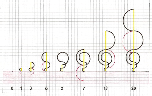
According to this sequence first few elements are- 0, 1, 3, 6, 2, 7, 13, 20, 12, 21, 11, 22, 10, 23, 9, 24, 8, 25, 43, 62, 42, 63, 41, 18, 42, 17, 43, 16, 44, 15, 45, 14, 46, 79, 113, 78, 114, 77, 39, 78, 38, 79, 37, 80, 36, 81, 35, 82, 34, 83, 33, 84, 32, 85, 31, 86, 30, 87, 29, 88, 28, 89, 27, 90, 26, 91, 157, 224…
The sequence satisfies
This is not a permutation of the integers: the first repeated term is Another one is Neil Sloane has conjectured that every number eventually appears, but it has not been proved. Even though 1015 terms have been calculated (in 2018), the number 852,655 has not appeared on the list.
Credits: On-Line Encyclopedia of Integer Sequences (OEIS) MATLAB CODE FOR Recamán Sequence
n=65; % Number of Terms in the Sequence
A = zeros(1,n);
A(1) = 0;
for ii = 1:n-1 % Algorithm to create the sequence
b = A(ii)-ii;
A(ii+1) = b + 2*ii;
if b > 0 && ~any(A == b)
A(ii + 1) = b;
end
end
hold on;
axis equal;
for i = 2:1:n % Plotting the Graphs
y = 0; x = (A(i)+A(i-1))/2; r = (A(i)-A(i-1))/2;
th = 0:pi/50:pi;
if A(i)>A(i-1)
xunit = r * cos(th) + x;
yunit = r * sin(th) + y;
end
if A(i)<A(i-1)
xunit = -r * cos(th) + x;
yunit = -r * sin(th) + y;
end
if mod(i,2) == 0
h = plot(xunit, -yunit,'k');
else
h = plot(xunit, yunit,'k');
end
end

MATLAB PLOT Gödel’s Incompleteness Theorems
“In Mathematics there is no ignorabimus. We must know, we shall know.”
-David HilbertThe incompleteness theorem, says roughly the following: under certain conditions in any language there exist true but unprovable statements.
The Set of True Statements– We assume that we are given a subset T of the set L (where L is the alphabet of the language under consideration) which is called the set of “true statements” (or simply “truths”). In going right to the subset T we are omitting such intermediate steps as: firstly, specifying which words of all the possible ones in the alphabet L are correctly formed expressions in the language, i.e.. have a definite meaning in our interpretation of the language (for example, 2 + 3, x + 3, x = y, x = 3, 2 = 3, 2 = 2 ‘are correctly formed expressions, while + = x is not); secondly, which of all the expressions are formulas, i.e., in our interpretation make statements which may depend on a parameter (for example, x = 3, x = y, 2 = 3, 2 = 2); thirdly, specifying which of all the possible formulas are closed formulas, i. e., statements which do not depend on parameters (for example, 2 = 3, 2 = 2); and finally, which of all the possible closed formulas are true statements (for example, 2 = 2).
Attempts at a Precise Formulation of the Incompleteness
Theorem.First Attempt– “Under certain conditions, given a fundamental pair (L, T) and a deductive system (P, P, B) over L, there always exists a word in T which does not have a proof.” This statement is still too vague. In particular, we could obviously think up many deductive systems having very few provable words. For example, there are no provable words at all in the empty deductive system (where P = 0).
Second Attempt– There is another more natural approach. Suppose we are given a language, in the precise meaning that we are given a fundamental pair (L, T). We now look for a deductive system over L (intuitively, we look for techniques of proof) in which we can prove as many words in T as possible, ideally, all words in T. Gödel’s theorem describes a situation in which such a deductive system (in which every word of T has a proof) does not exist. Thus, we would like to make the following statement: “Under certain conditions concerning the fundamental pair (L, T) there does not exist a deductive system over L in which every word in T has a proof.” However, this statement is clearly false, since one need only take the deductive system with P = L, P = P” and ~ (p) = p for all p in P”: then every word in L is trivially provable. Thus, we need a restriction on the deductive systems that we are allowed to use.

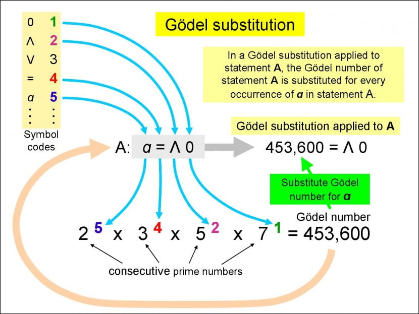
Code devised by Gödel for every mathematical symbol in the system correspond to a unique natural number and every formula to generate a unique natural number called a Gödel number using prime numbers in the manner shown. A Gödel substitution is defined by plugging the Gödel number back into the formula wherever we find the symbol “ɑ”. The Simplest Incompleteness Criteria
We now know that enumerability of the set T is equivalent to the existence of a complete and consistent deductive system for (L, T). However, we might be interested not in all truths in the language, but only in truths of a certain type or a certain class, much as a student studying for a math exam is not concerned with the truth of all mathematical statements, but only those which are likely to be encountered on the exam. For example, we might want to construct a deductive system in which one can derive all true statements of length at most 1000 and cannot derive any false statement of length at most 1000. In this case, for a statement of length greater than 1000 the question of whether or not it can be derived in the deductive system may have nothing- to do with whether or not it is true. Moreover, in certain situations (such as the language of set theory), one cannot even define the set of all truths in their totality. This is why we restrict ourselves to considering consistency and completeness for subsets of the word set L.There are three axioms of Gödel’s Incompleteness Theorems which I will try to provige through another post.


 wouldn’t be totally convex.


. Public domain.")


![{\begin{aligned}3\varphi ^{3}-5\varphi ^{2}+4&=3(\varphi ^{2}+\varphi )-5\varphi ^{2}+4\\&=3[(\varphi +1)+\varphi ]-5(\varphi +1)+4\\&=\varphi +2\approx 3.618.\end{aligned}}](https://wikimedia.org/api/rest_v1/media/math/render/svg/49ad0d344bfe44a351629cea9fefc61e93c90d92)

 is the kth Fibonacci number.
 , with basis


 This is not a permutation of the integers: the first repeated term is
  Another one is