Ricci Flow
“As far as the laws of mathematics refer to reality, they are not certain;
-Albert Einstein
and as far as they are certain, they do not refer to reality.“In 1900, Henri Poincare put for a conjecture that colloquially states that
“If it walks like a sphere and it quacks like a sphere, it is a sphere.” This statement, known as the Poincare conjecture, became one of the early questions in a field now called “low-dimensional topology” and proved itself to be extremely subtle and intractable. It attracted the attention of many great mathematicians and attempts to solve it lead to the development of powerful tools.In the early 1980s, Richard Hamilton put forth an ambitious program to
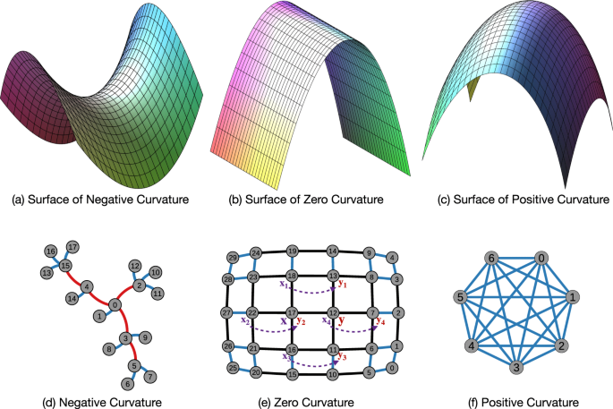
attack the Poincare conjecture. He proposed a process called the Ricci flow that would deform the shape of a space and hopefully allow its curvature to dissipate throughout the space. If the space satisfied the hypotheses of the Poincare conjecture, he hoped the space would evolve into a round sphere and that he could prove the conjecture with this nicer space. He was able to make this approach work in two dimensions as a proof of concept, but he found that in three dimensions the flow would sometimes violently rip apart spaces and so was unable to finish the proof.The rest of the story is already a part of mathematical lore.
The Intuition–
If there is no heat source the hottest points of any surface will cool down while the coldest ones warm up. This phenomena has been studied using the heat equation, which was introduced by Joseph Fourier. This equation says that a heat distribution u will evolve over time via the equation ∂u/∂t = ∆u.
The Laplacian–
The above equation involves the Laplacian ∆u. Many of you will remember this from vector calculus as being ∇·(∇u) (or div(grad u)) but it is illustrative to think of it in terms of coordinates, where we have (in R3) ∆u = ∂2u/∂x2 + ∂2u/∂y2 + ∂2u/∂z2 .
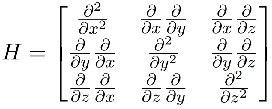
However, for the context of the Ricci flow, we can consider the Hessian matrix,

Then from this matrix we can see that the Laplacian ∆u = tr H(u). The Heat Equation–
The heat equation is a partial differential equation given by the expression ∂u/∂t = ∆u. We think of t as being a time parameter and the right hand side as being derivatives in space. Given an initial distribution of heat a solution to this equation will give the temperature of points at a time t. We call such a solution a “heat flow.”

Background material from Ricci flow–
Hamilton introduced the Ricci flow equation, ∂g(t)/∂t = −2Ric(g(t)). This is an evolution equation for a one-parameter family of Riemannian metrics g(t) on a smooth manifold M. The Ricci flow equation is weakly parabolic and is strictly parabolic modulo the ‘gauge group’, which is the group of diffeomorphisms of the underlying smooth manifold. One should view this equation as a non-linear, tensor version of the heat equation. From it, one can derive the evolution equation for the Riemannian metric tensor, the Ricci tensor, and the scalar curvature function. These are all parabolic equations. For example, the evolution equation for scalar curvature R(x,t) is ∂R/∂t (x,t) = △R(x,t) + 2|Ric(x,t)|^2, illustrating the similarity with the heat equation.
For a better understanding I would recommend an understanding of the Riemannian metric tensor.
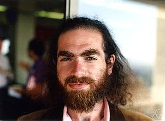
Grigori Perelman’s advances–

Grigori Perelman So far we have been discussing the results that were known before Perelman’s work. They concern almost exclusively Ricci flow (though Hamilton in had introduced the notion of surgery and proved that surgery can be performed preserving the condition that the curvature is pinched toward positive). Perelman extended in two essential ways the analysis of Ricci flow – one involves the introduction of a new analytic functional, the reduced length, which is the tool by which he establishes the needed non collapsing results, and the other is a delicate combination of geometric limit ideas and consequences of the maximum principle together with the non collapsing results in order to establish bounded curvature at bounded distance results. These are used to prove in an inductive way the existence of canonical neighborhoods, which is a crucial ingredient in proving that is possible to do surgery iteratively, creating a flow defined for all positive time. While it is easiest to formulate and consider these techniques in the case of Ricci flow, in the end one needs them in the more general context of Ricci flow with surgery since we inductively repeat the surgery process, and in order to know at each step that we can perform surgery we need to apply these results to the previously constructed Ricci flow with surgery. We have chosen to present these new ideas only once – in the context of generalized Ricci flows – so that we can derive the needed consequences in all the relevant contexts from this one source.
Grigori Perelman was offered The Fields Medal and one million dollars as promised by the Clay Mathematical Institute for proving the Poincare Conjecture using Ricci Flow. However he turned down the offer very humbly.
Bessel’s Function
Just imagine a dew drop falling from a leaf on the surface of an absolutely calm lake, creating short ripples in water which then fight among themselves and disappear in time. Such an amazing thing to watch but, today we will unfold the mathematics behind it.
The function which defines the phenomenon stated above or any acoustic activity on a circular membrane (exploited by most of the musical instruments) is called the Bessel’s function in the honour of the German astronomer Friedrich Wilhelm Bessel.
The Bessel function was first defined by famous mathematician Daniel Bernoulli and then generalized by Friedrich Bessel during an investigation of solutions of one of Kepler’s equations of planetary motion.
Bessel functions are used to solve in 3-D the wave equation at a given (harmonic) frequency. The solution is generally a sum of spherical Bessel’s functions that gives the acoustic pressure at a given location of the 3-D space.
The Bessel’s function is nothing but the canonical solutions of the Bessel’s differential equation-

for an arbitrary complex number α. Although α and −α produce the same differential equation, it is conventional to define different Bessel functions for these two values in such a way that the Bessel functions are mostly smooth functions of α. The most important cases are when α is an integer or half-integer.
The Bessel’s function can be categorized as follows-
TYPE FIRST KIND SECOND KIND Bessel functions Jα Yα Modified Bessel functions Iα Kα Hankel functions H(1)α = Jα + iYα H(2)α = Jα − iYα Spherical Bessel functions jn yn Spherical Hankel functions h(1)n = jn + iyn h(2)n = jn − iyn Bessel functions of the first kind of order n and -n –
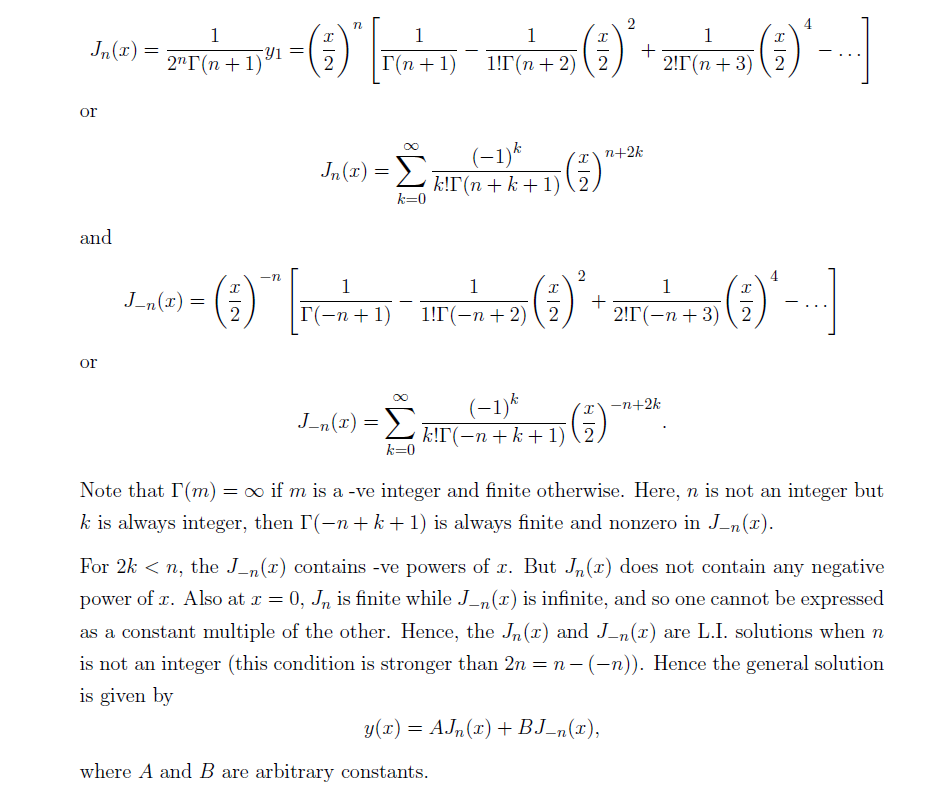
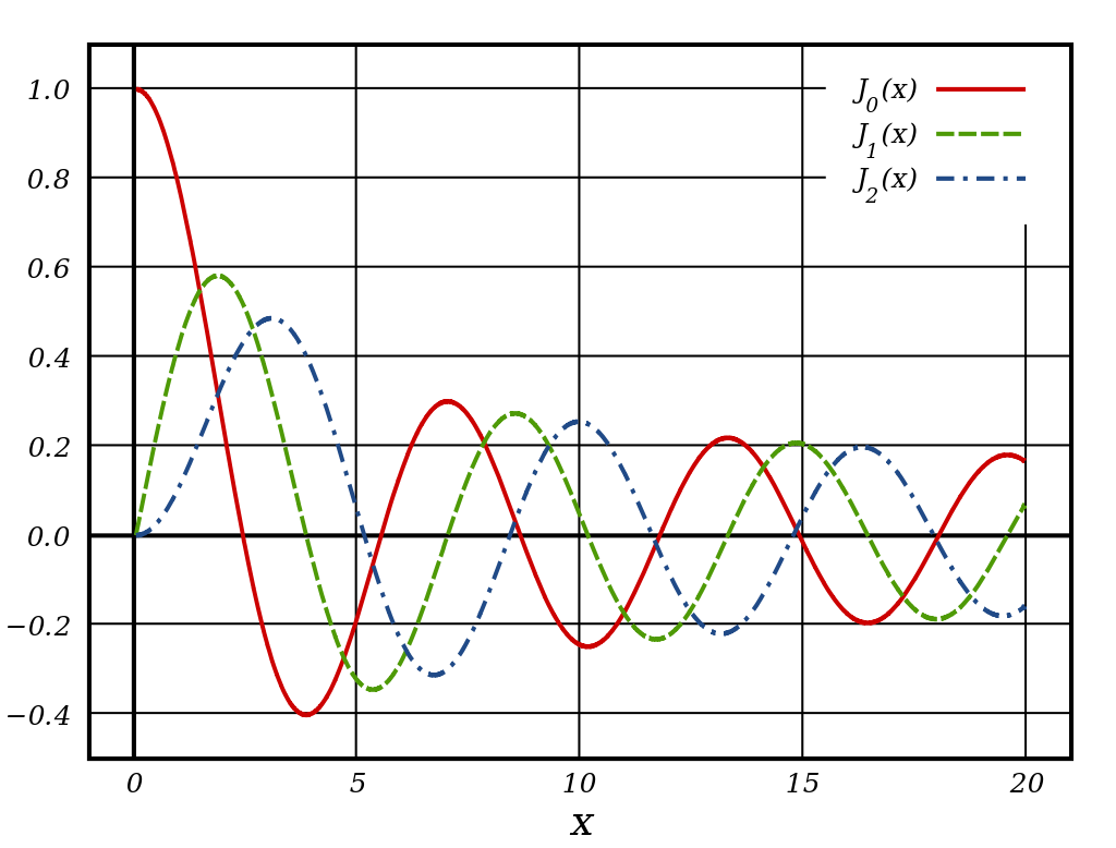
We define the Bessel functions of the first kind as-


Graph of Bessel’s Function of First Kind Bessel’s Function has a wide range of application in electromagnetic wave theory, solution to the radial Schrödinger equation (in spherical and cylindrical coordinates) for a free particle and many more. We will try understand few of them in the days to come.
The Collatz Conjecture

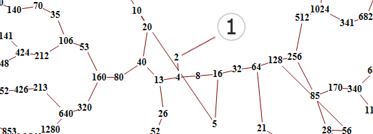
Collatz Conjecture Art Lets take a positive integer.
If the chosen number is even then just divide it by 2. If the chosen number is odd triple it and add 1. Now keep applying these rules repeatedly.
Statement:- This process will eventually reach the number 1, regardless of which positive integer is chosen initially.
In notation:

(that is: ai is the value of f applied to n recursively i times; ai = fi(n)).
That smallest i such that ai = 1 is called the total stopping time of n. The conjecture asserts that every n has a well-defined total stopping time. If, for some n, such an i doesn’t exist, we say that n has infinite total stopping time and the conjecture is false. If the conjecture is false, it can only be because there is some starting number which gives rise to a sequence that does not contain 1. Such a sequence would either enter a repeating cycle that excludes 1, or increase without bound. No such sequence has been found.
For example starting with 12 we get the sequence 12, 6, 3, 10, 5, 16, 8, 4, 2, 1.
The sequence of numbers involved is sometimes referred to as the hailstone sequence or hailstone numbers (because the values are usually subject to multiple descents and ascents like hailstones in a cloud), or as wondrous numbers.
“Mathematics may not be ready for such problems.”- Paul Erdős

All Returns To 1 Defining the Collatz function f(x) as follows:

If x is a positive integer, then f(x) is the next number after x in its Collatz sequence.
To extend this function to the real numbers, simply recall that (-1)x = cos(πx). In fact, this gets us an extension to the complex numbers at the same time, and after some simplification we arrive at:

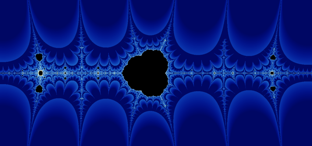
It is a holomorphic function and we can study the fractal that its iterates induce.

Collatz Fractals The fractal is located on the complex plane, and the horizontal line through the middle of the image is the real line. Black regions are regions in which the orbit of that number is bounded, while other colors indicate that the orbit of that number is unbounded (notice the large region of bounded numbers around z = 0). The big “spikes” that occur along the real line are, as we would expect, located at the integers (the image above is wide enough that you can see the spikes at z = -2, -1, 1, and 2).
The Collatz Conjecture is quite intimately connected with deep roots of nature and much more lies in the dark left to discovered about it which includes a PROOF.
Fascinating Quaternions
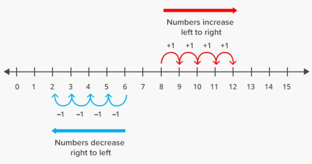
Let us imagine taking strolls in One Dimension. Well we seem to only move forward and backward along a single line in a fixed direction. We can imagine walking along the real number line. Now if we represent our position in this situation we would be using One Dimensional numbers.

The number line representing 1-D numbers. Now lets move onto a Two Dimensional walk. We can simply represent these as moving around in a flat plane with definite X and Y axes to pin point our position. The question arises, ‘Can we denote our position by a single number?’ The answer is fascinating in itself because with this we delve into probably the most interesting space of numbers. The position in 2-D is represented by complex numbers. Its a very simple concept to denote a number using two directions to reach it from any other number.

Travelling in a complex plane is very simple. We have to select an initial position first. Lets talk about this example and select the initial position as the origin. Then moving a unit in positive x-direction, pausing for a while and then taking a counter-clockwise turn of 90 degrees and moving another unit but now in positive y-direction. We have reached (1+i). Its just like another number, we can add two of them together and multiply also. For example lets add up (1+i) and (-1+i) we get 2i on the positive y-axis. Again lets multiply i and (1+i). Now here is a little catch. What is ‘i’ we are talking so much about? Its called ‘iota’ which represents the square root of negative 1 [(-1)^(1/2)]. So if we multiply ‘i’ to itself we get back negative one. Lets check for ourselves, multiplying i and 1+i, we get i*(1+i)=i*1+i*i=i-1=-1+i. We turn 90 degrees counter-clockwise from (1+i) ending up in (-1+i). Hence we see that rotation is feasible.
Now the real deal, to represent a single number for three dimensions.
By now many of you are thinking that if we can represent a 2-D number by ‘a+ib’ form then quite intuitively a 3-D number can be represented by something of the form ‘a+ib+jc’. Well it is a 3-D number but we cannot use it to move about in 3-D space. But here is where we get to see a brilliant mathematical mind excel.
The advent of Quaternions.
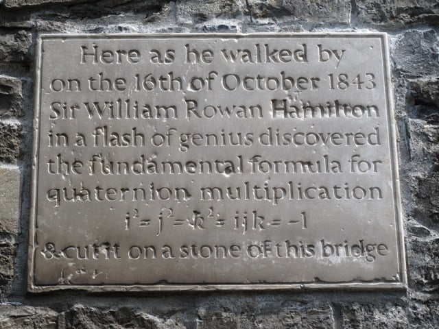
One fine day Sir William Rowan Hamilton was taking strolls by a canal with his wife and the same question was hovering in his mind “How to represent a position in 3-D using 3-D number?” Then he was struck by an idea and he ran to a bridge over the canal and engraved his findings which now has been developed into an embedded stone carving.

The mind blowing idea was to use four dimensions to define a position and to move about in 3-D. Hence, the formula Sir Hamilton came up with was quite similar to the concept of complex numbers is as stated below- i^2=j^2=k^2=i*j*k=-1. Simple yet brilliant. This theorem gained massive popularity as it opens up a vast field to work with. Now that we know that these are actually 4-D so the number can be written as ‘a+ib+cj+dk’. We can now freely rotate and move about in 3-D. Suppose we take a point P(xi+yj+zk) in a 3-D plane. We need h=a+bi+cj+dk and h*=a-bi-cj-dk. The changed coordinates will be P*= h x P x h*.
Like the Quaternions there are Octonions but as we go up these lose some properties and become quite faint and is not studied widely.
The Hemchandra Sequence
Mathematics in early days was seen as some kind of tool to make particular art forms perfect and in sync with nature. Now here comes the story of perfecting the art of poetry from 11th century India. Acharya Hemchandra Suri born in 1088 AD was a prodigy in himself to have expanded in vast fields like Grammar, Poetry, Lexicography, and most famously Mathematics. As we are particularly interested in mathematics I must acknowledge his enormous achievement in this area. Hemchandra described the Fibonacci sequence in 1150 AD fifty years before Fibonacci himself. He was considering a sequence of notes of length n, and he showed that these could be formed by adding a short syllable to a note of length n − 1, or a long syllable to one of n − 2. The recursion relation F(n)= F(n-1) +F(n-1) represents the Fibonacci sequence. Hemchandra studied the rhythms of Sanskrit poetry. Syllables in Sanskrit are either long or short. Long syllables have twice the length of short syllables. The question he asked is ‘How many rhythm patterns with a given total length can be formed from short and long syllables?’ And this led to a revolution of beats and rhythms and even mathematics.

In the sunflower, individual
flowers are arranged along
curved lines which rotate
clockwise and counterclockwise.
Credits: The Fibonacci sequence in phyllotaxis.
– Laura Resta (Degree Thesis in Bio-mathematics)