Oscillatory integrals in one form or another have been an essential part of harmonic analysis from the very beginnings of that subject. Besides the obvious fact that the Fourier transform is itself an oscillatory integral par excellence, one need only recall the occurrence of Bessel functions in the work of Fourier, the study of asymptotic related to these functions by Airy, Stokes, and Lipschitz, and Riemann’s use of the method of “stationary phase” in finding the asymptotic of certain Fourier transforms, all of which took place well over 100 years ago.
A basic problem which comes up whenever performing a computation in harmonic analysis is how to quickly and efficiently compute (or more precisely, to estimate) an explicit integral. Of course, in some cases undergraduate calculus allows one to compute such integrals exactly, after some effort (e.g. looking up tables of special functions), but since in many applications we only need the order of magnitude of such integrals, there are often faster, more conceptual, more robust, and less computationally intensive ways to estimate these integrals.
The dyadic decomposition of a function
Littlewood–Paley theory uses a decomposition of a function f into a sum of functions fρ with localized frequencies. There are several ways to construct such a decomposition; a typical method is as follows. If f(x) is a function on R, and ρ is a measurable set (in the frequency space) with characteristic function Xρ(ξ), then fρ is defined via its Fourier transform fρ := Xρ . Informally, fρ is the piece of f whose frequencies lie in ρ. If Δ is a collection of measurable sets which (up to measure 0) are disjoint and have union on the real line, then a well behaved function f can be written as a sum of functions fρ for ρ ∈ Δ. When Δ consists of the sets of the form ρ = [-2k+1,-2k] U [2k, 2k+1] for k an integer, this gives a so-called “dyadic decomposition” of f : Σρ fρ. There are many variations of this construction; for example, the characteristic function of a set used in the definition of fρ can be replaced by a smoother function. A key estimate of Littlewood Paley theory is the Littlewood–Paley theorem, which bounds the size of the functions fρ in terms of the size of f. There are many versions of this theorem corresponding to the different ways of decomposing f. A typical estimate is to bound the Lp norm of (Σρ |fρ|2)1/2 by a multiple of the Lp norm of f. In higher dimensions it is possible to generalize this construction by replacing intervals with rectangles with sides parallel to the coordinate axes. Unfortunately these are rather special sets, which limits the applications to higher dimensions.
In the case where the integral to evaluate is non-negative, e.g.
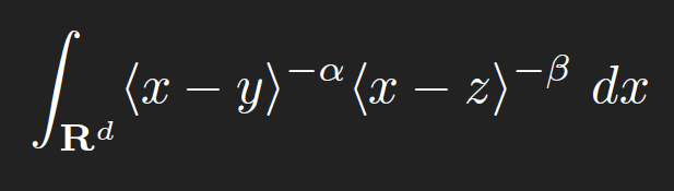
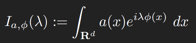
then the method of decomposition, particularly dyadic decomposition, works quite well: split the domain of integration into natural regions, such as dyadic annuli on which a key term in the integrand is essentially constant, estimate each sub-integral (which generally reduces to the geometric problem of measuring the volume of some standard geometric set, such as the intersection of two balls), and then sum (generally one ends up with summing a standard series such a geometric series or harmonic series). For non-negative integrands, this approach tends to give answers which only differ above and below from the truth by a constant (possibly depending on things such as the dimension d). Slightly more generally, this type of estimation works well in providing upper bounds for integrals which do not oscillate very much. With some more effort, one can often extract asymptotics rather than mere upper bounds, by performing some sort of expansion (e.g. Taylor expansion) of the integrand into a main term (which can be integrated exactly, e.g. by methods from undergraduate calculus), plus an error term which can be upper bounded by an expression smaller than the final value of the main term. However, there are many cases in which one has to deal with integration of highly oscillatory integrands, in which the naive approach of taking absolute values (thus destroying most of the oscillation and cancellation) will give very poor bounds. A typical such oscillatory integral takes the form
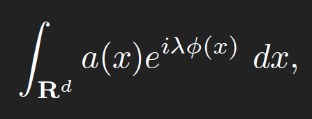
where a is a bump function adapted to some reasonable set B (such as a ball), Φ is a real -valued phase function (usually obeying some smoothness conditions), and λ ∈ R is a parameter to measure the extent of oscillation. One could consider more general integrals in which the amplitude function a is replaced by something a bit more singular, e.g. a power singularity |x|−α, but the aforementioned dyadic decomposition trick can usually decompose such a “singular oscillatory integral” into a dyadic sum of oscillatory integrals of the above type. Also, one can use linear changes of variables to rescale B to be a normalised set, such as the unit ball or unit cube. In one dimension, the definite integral

is also of interest, where J is now an interval. While one can dyadically decompose around the endpoints of these intervals to reduce this integral to the previous smoother integral, in one dimension one can often compute the integrals more directly.
One dimensional theory
Beginning with the theory of the one-dimensional definite integrals,
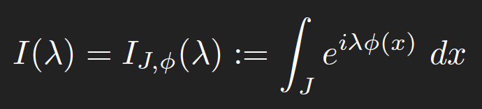
where J is an interval, λ ∈ R, and Φ : J → R is a function (which we shall assume to be smooth, in order to avoid technicalities). We observe some simple invariances:
• I(−λ) = I(λ), thus negative λ and positive λ behave similarly;
• Subtracting a constant from λ does not affect the magnitude of I(λ);
• If L : R → R is any invertible affine-linear transformation, then IL(J),Φ◦L−1(λ) =| det(L)|IJ,Φ(λ).
• We haveIJ,Φ(λ) = IJ,Φ(1).
From the triangle inequality we have the trivial bound |I(λ)| ≤ |J|.
This bound is of course sharp if Φ is constant. But if Φ is non-constant, we expect I(λ) to decay as λ → ±∞.
Higher dimensional theory
The higher dimensional theory is less precise than the one-dimensional theory, mainly because the structure of stationary points can be significantly more complicated. Nevertheless, we can still say quite a bit about the higher dimensional oscillatory integrals
in many cases. The van der Corput lemma becomes significantly weaker, and will not be discussed here; however, we still have the principle of non stationary phase.
Principle of non-stationary phase
Let a ∈ C0∞ (Rd), and let Φ : Rd → R be smooth such that ∇Φ is non-zero on the support of a. Then Ia,Φ(λ) =ON,a,Φ,d(λ−N) for all N ≥ 0.
Adapted from LECTURE NOTES by TERENCE TAO. No copyright infringement intended.