
The Laplace transform takes a function of time and transforms it to a function of a complex variable s. As the transform is invertible, no information is lost and it is quite reasonable to think of a function f(t) and its Laplace transform F(s) as two aspects of the same phenomenon. Each view has its uses and some features of the phenomenon are easier to understand in one view or the other.We can use the Laplace transform to transform a linear time invariant system from the time domain to the s-domain.
One important feature of the Laplace transform is that it can transform analytic problems to algebraic problems. We will see examples of this for differential equations.
Definition– The Laplace transform of a function f(t) is defined by the integral

for all s where the integral converges. Here s is allowed to take complex values. The Laplace Transform is only concerned with f(t) for t > 0. Generally, speaking we can require f(t) = 0 for t < 0.
Examples-
Let f(t) = e^at. Compute F(s) = L(f; s) directly. Give the region in the
complex s-plane where the integral converges.

The last formula comes from plugging infinity into the exponential. This is 0 if Re(a – s) < 0 and undefined otherwise.
Connection to Fourier transform–
The Laplace and Fourier Transforms are intimately connected. The Laplace Transform is often called Fourier – Laplace Transform. to see the connection we will start with the Fourier Transform of a function f(t).
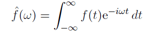
If we assume f(t) = 0 for t<0, this becomes
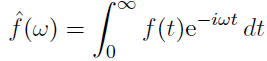
Now if s = iw then the Laplace Transform is

Comparing these two equations we see that f(w) = L(f; iw). We see transforms are basically the same things different notations at least for functions that are 0 for t<0.
Exponential Type
The Laplace transform is defined when the integral for it converges. Functions of exponential type are a class of functions for which the integral converges for all s with Re(s) large enough.
Definition. We say that f(t) has exponential type a if there exists an M such that |f(t)|<Me^at for all t>0.
Properties of Laplace Transform
Property 1. The Laplace transform is linear. That is, if a and b are constants and f and g are functions then L(af + bg) = aL(f) + bL(g).
Property 2. A key property of the Laplace transform is that, with some technical details, Laplace transform transforms derivatives in t to multiplication by s (plus some details). This is proved in the following theorem.
Theorem. If f(t) has exponential type a and Laplace transform F(s) then L(f'(t); s) = sF(s) – f(0); valid for Re(s) > a.
Proof. We prove this using integration by parts.

In the last step we used the fact that at t = ∞ , f(t)e^-(st) = 0, which follows from the assumption about exponential type.
L(f”; s) = (s^2) F(s) – sf(0) – f'(0)
L(f”’; s) = (s^3)F(s) – (s^2)f(0) – sf'(0) – f”(0)
Property 3. Theorem. If f(t) has exponential type a, then F(s) is an analytic function for Re(s) > a and
F'(s) = -L(t f(t); s).
Proof. We take the derivative of F(s). The absolute convergence for Re(s) large guarantees that we can interchange the order of integration and taking the derivative.

This is called the s-derivative rule. We can extend it to more derivatives in s: Suppose L(f; s) = F(s). Then,

Example- Use the s-derivative rule and the formula L(1; s) = 1/s to compute the transform of t^n for n a positive integer.
Let f(t) = 1 and F(s) = L(f; s). Using the s-derivative rule we get

Property 4. T- shift rule. Assume f(t) = 0 for t<0. Suppose a>0. Then, L(f(t-a); s) = e^-(as)F(s).
Proof. We go back to the definition of the Laplace Transform and make the change of variables T = t – a.

Laplace Inverse
There are many functions with the same Laplace Transform, so we need to check whether the inverse function holds or not. We list some of the ways this can happen.
- If f(t) = g(t) for t>0, then clearly F(s) = G(s). Since the Laplace Transform only concerns t>0, the functions can differ completely for t<0.
- Suppose f(t) = e^at and
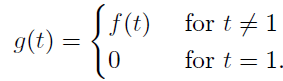
That is, f and g are the same except we arbitrarily assigned them different values at t = 1. Then, since the integrals won’t notice the difference at one point, F(s) = G(s) = 1 = 1/(s – a). In this sense it is impossible to define L^-(1)(F) uniquely. The inverse exists as long as we consider two functions that only differ on a negligible set of points the same.
Theorem. Suppose f and g are continuous and F(s) = G(s) for all s with Re(s)> a for some a. Then f(t) = g(t) for t > 0.
This theorem can be stated in a way that includes piecewise continuous functions. Such a statement takes more care, which would obscure the basic point that the Laplace Transform has a unique inverse up to some, for us, trivial differences.
Theorem. Laplace inversion 1. Assume f is continuous and of exponential type a. Then for c > a we have
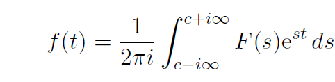
This formula holds for t>0.
Theorem. Laplace inversion 2. Suppose F(s) has a finite number of poles and decays like 1/s (or faster).

Then L(f; s) = F(s).