Green’s functions are named after the British mathematician George Green, who first developed the concept in the 1820s. In the modern study of linear partial differential equations, Green’s functions are studied largely from the point of view of fundamental solutions instead.
The term is also used in physics, specifically in quantum field theory, aerodynamics, aeracoustics, electrodynamics, seismology and statistical field theory, to refer to various types of correlation functions, even those that do not fit the mathematical definition. In quantum field theory, Green’s functions take the roles of propagators.
Preliminary ideas and motivation
The delta function
Definition- The δ-function is defined by the following three properties,
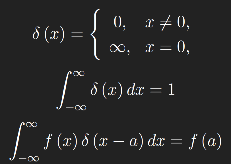
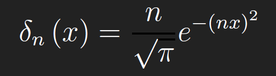
where f is continuous at x = a. The last is called the shifting property of the δ-function. To make proofs with the δ-function more rigorous, we consider a δ-sequence, that is, a sequence of functions that converge to the δ-function, at least in a pointwise sense. Consider the sequence
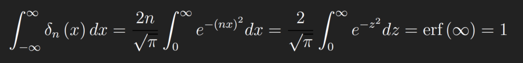
Note that,
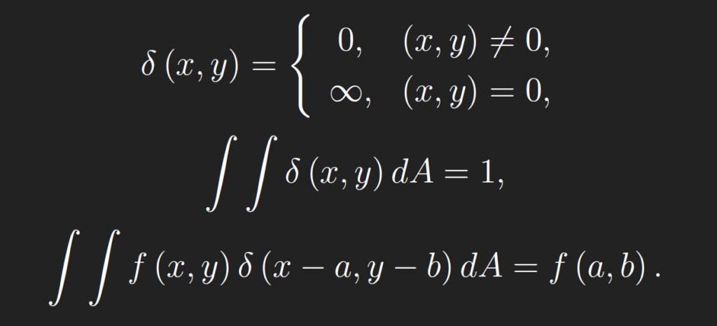
The 2D δ-function is defined by the following three properties,
Finding the Green’s function
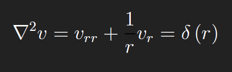
To find the Green’s function for a 2D domain D, we first find the simplest function that satisfies ∇2v = δ(r). Suppose that v (x, y) is axis-symmetric, that is, v = v (r). Then
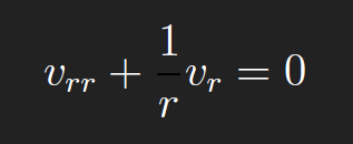
For r > 0,
Integrating gives
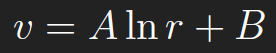
For simplicity, we set B = 0. To find A, we integrate over a disc of radius ε centered at(x, y),Dε,
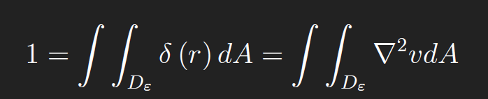
From the Divergence Theorem, we have
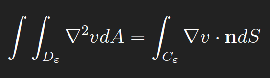
where Cε is the boundary of Dε, i.e. a circle of circumference 2πε. Combining the previous two equations gives
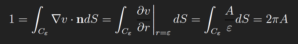
Hence
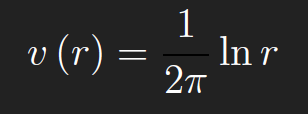
This is called the fundamental solution for the Green’s function of the Laplacian on 2D domains. For 3D domains, the fundamental solution for the Green’s function of the Laplacian is −1/(4πr), where r = (x − ξ)2 + (y − η)2 + (z − ζ)2. The Green’s function for the Laplacian on 2D domains is defined in terms of the corresponding fundamental solution,
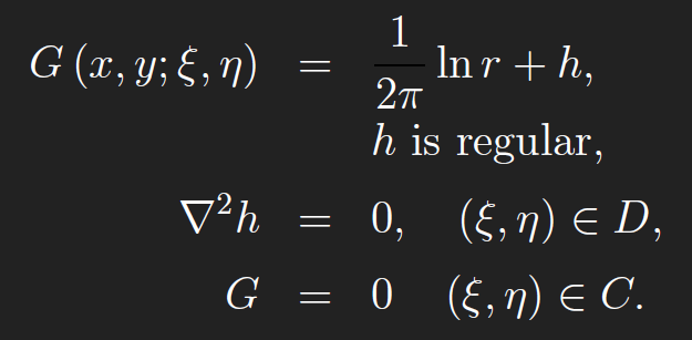
The term “regular” means that h is twice continuously differentiable in(ξ, η)on D. Finding the Green’s function G is reduced to finding a C2 function h on D that satisfies
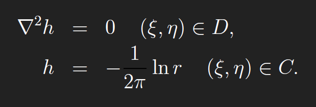
The definition of G in terms of h gives the BVP for G. Thus, for 2D regions D, finding the Green’s function for the Laplacian reduces to finding h.
Examples


Plot of the Green’s function G(x,y;ξ,η)for the Laplacian operator in the upper half plane, for(x, y)=(√2,√2).
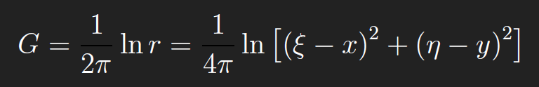
(i) Full plane D = R2. There are no boundaries so h =0 will do, and
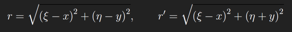
(ii)Half plane D = {(x, y): y> 0}. We find G by introducing what is called an “image point” (x, −y) corresponding to(x, y). Let r be the distance from (ξ,η) to (x, y)and r ′ the distance from(ξ,η) to the image point(x,−y),
Conformal mapping and the Green’s function
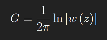
Conformal mapping allows us to extend the number of 2D regions for which Green’s functions of the Laplacian ∇2u can be found. We use complex notation, and let α = x + iy be a fixed point in D and let z = ξ + iη be a variable point in D (what we’re integrating over). If D is simply connected (a definition from complex analysis), then by the Riemann Mapping Theorem, there is a conformal map w (z)(analytic and one-to-one) from D into the unit disk, which maps α to the origin, w (α) =0 and the boundary of D to the unit circle, |w (z)|=1for z ∈∂D and0 ≤|w (z)|< 1 for z ∈D/∂D. The Greens function G is then given by
To see this, we need a few results from complex analysis. First, note that for z ∈∂D, w (z)=0 so that G = 0. Also, since w (z)is1-1, w (z)> 0for z = α. Thus, we
can write w (z) =(z −α)n H(z) where H(z) is analytic and nonzero in D. Since w (z)is1-1, w ′ (z)> 0 on D. Thus n =1. Hence w (z)=(z −α)H(z) and
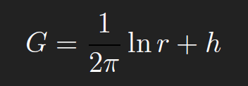
where,
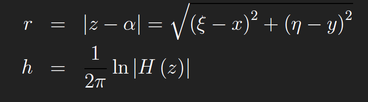
Since H(z) is analytic and nonzero in D, then (1/2π) lnH(z) is analytic in D and hence its real part is harmonic, i.e. h = ℜ ((1/2π) lnH(z)) satisfies ∇2h =0in D. Thus by our definition above, G is the Green’s function of the Laplacian on D.
NO COPYRIGHT INFRINGEMENT INTENDED