The hydrodynamics equations are nothing more than signal-propagation equations, and equations of this kind are called hyperbolic equations. The equations of hydrodynamics are only a member of the more general class of hyperbolic equations, and there are many more examples of hyperbolic equations than just the equations of hydrodynamics.
The simplest form of a hyperbolic equation
Consider the equation ∂tq + u∂xq = 0.
where q = q(x, t) is a function of one spatial dimension and time, and u is a velocity that is constant in space and time. This is called an advection equation, as it describes the time dependent shifting of the function q(x) along x with a velocity u. The solution at any time t > t0 can be described as a function of the state at time t0: q(x, t) = q(x − ut, 0).
This is a so-called initial value problem in which the state at any time t > t0 can be uniquely found when the state at time t = t0 is fully given. The characteristics of this problem are straight lines: xchar(t) = x(0)char + ut. This is a family of lines in the (x, t) plane, each of which is labeled by its own unique value of (x(0)char).

Hyperbolic sets of equations: the linear case with constant Jacobian
Let us consider a set of linear equations that can be written in the form:∂tQ + A∂xQ = 0, where Q is a vector of m components and A is an m × m matrix. This system is called hyperbolic if the matrix A is diagonalizable with real eigenvalues. The matrix is diagonalizable if there exists a complete set of eigenvectors ei, i.e. if any vector can be written as:
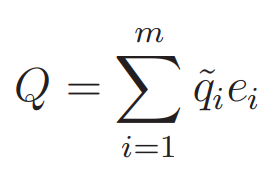
In this case one can write
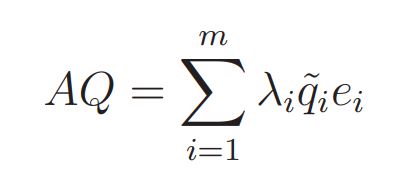
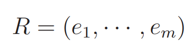
We can define a matrix in which each column is one of the eigenvectors:
Then we can transform the first equation into:
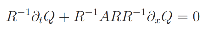
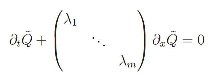
which with Q˜ = R−1Q then becomes:
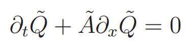
where A˜ = diag (λ1, ··· , λm). Not all λi must be different from each other. This system of equations has in principle m sets of characteristics. But any set of characteristics that has the same characteristic velocity as another set is usually called the same set of characteristics. So in the case of 5 eigenvalues, of which three are identical, one typically says that there are three sets of characteristics.
Hyperbolic equations: the non-linear case
Let us focus on the general conservation equation:

where, as ever, Q = (q1, ··· , qm) and F = (f1, ··· , fm). In general, F is not always a linear function of Q, i.e. it cannot always be formulated as a matrix A times the vector Q (except if A is allowed to also depend on Q, but then the usefulness of writing F = AQ is a bit gone). So let us assume that F is some non-linear function of Q. Let us, for the moment, assume that F = F(Q, x) = F(Q), i.e. we assume that there is no explicit dependence of F on x, except through Q. Then we get
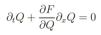
where ∂F/∂Q is the Jacobian matrix, which depends, in the non-linear case, on Q itself. We can nevertheless decompose this matrix in eigenvectors (which depend on Q) and we obtain
Here the eigenvalues λ1, ··· , λm and eigenvectors (and hence the meaning of Q˜) depends on Q. In principle this is not a problem. The characteristics are now simply given by the state vector Q itself. The state is, so to speak, self-propagating. We are now getting into the kind of hyperbolic equations like the hydrodynamics equations, which are also non-linear self-propagating.