The Hankel transform is an integral transform and was first developed by the mathematician Hermann Hankel. It is also known as the Fourier–Bessel transform. Just as the Fourier transform for an infinite interval is related to the Fourier series over a finite interval, so the Hankel transform over an infinite interval is related to the Fourier–Bessel series over a finite interval. In mathematics, the Hankel transform expresses any given function f(r) as the weighted sum of an infinite number of Bessel functions of the first kind Jν(kr). The Bessel functions in the sum are all of the same order ν, but differ in a scaling factor k along the r axis. The necessary coefficient Fν of each Bessel function in the sum, as a function of the scaling factor k constitutes the transformed function.
Definition of the Hankel Transform
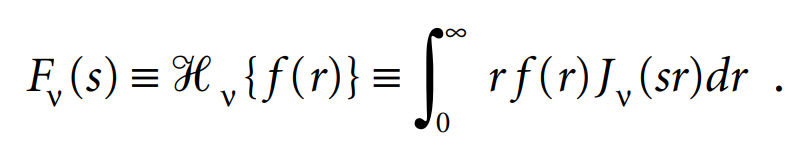
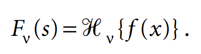
Let ƒ(r) be a function defined for r ≥ 0. The vth order Hankel transform of ƒ(r) is defined as
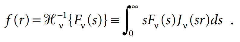
If v > –1/2, Hankel’s repeated integral immediately gives the inversion formula
The most important special cases of the Hankel transform correspond to v = 0 and v = 1. Sufficient but not necessary conditions for the validity
- f (r) = O(r –k), r → ∞ where k > 3/2.
- f ′(r) is piecewise continuous over each bounded subinterval of [0, ∞).
- f(r) is defined as [f(r+) + f(r–)]/2.
Connection with the Fourier Transform
We consider the two-dimensional Fourier transform of a function ϕ(x,y), which shows a circular symmetry. This means that ϕ(r cos θ, r sin θ) ƒ(r,θ) is independent of θ. The Fourier transform of ϕ is
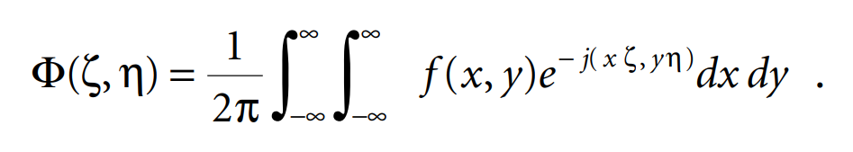
We introduce the polar coordinates x = rcosθ, y = rsin θ, and ζ = scosϕ, η = ssinϕ.
We have then
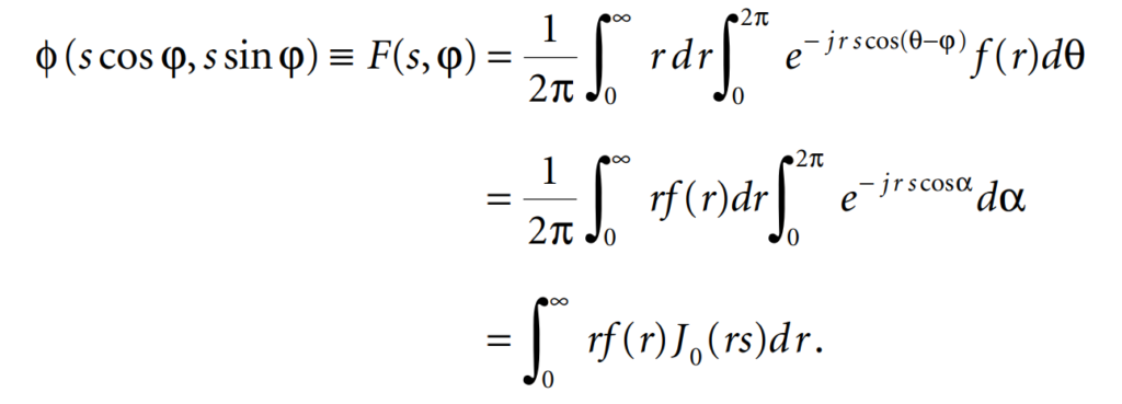
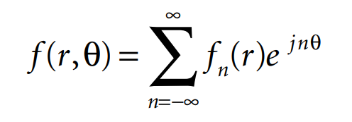
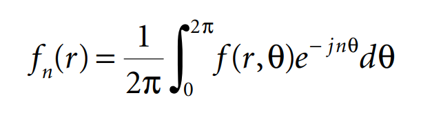
This result shows that F(s,ϕ) is independent of ϕ, so that we can write F(s) instead of F(s, ϕ). Thus, the two-dimensional Fourier transform of a circularly symmetric function is, in fact, a Hankel transform of order zero. This result can be generalized: the N-dimensional Fourier transform of a circularly symmetric function of N variables is related to the Hankel transform of order N/2 – 1. If ƒ(r,θ) depends on θ, we can expand it into a Fourier series
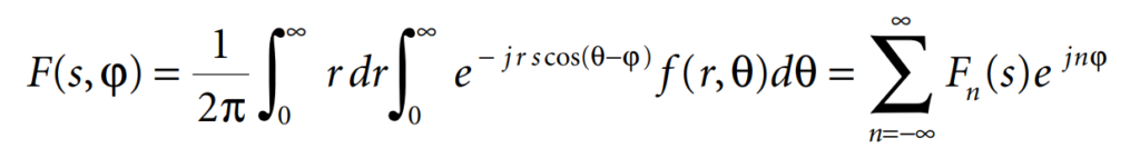
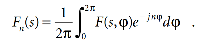
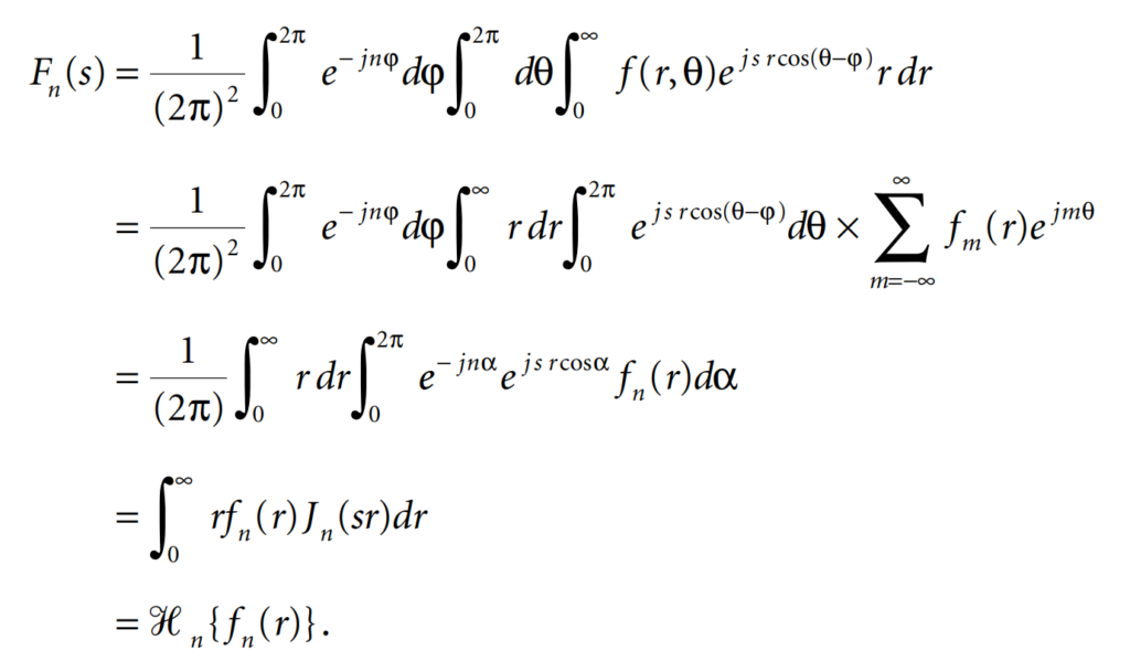
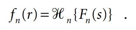
In a similar way, we can derive
Properties
Hankel transforms do not have as many elementary properties as do the Laplace or the Fourier transforms. For example, because there is no simple addition formula for Bessel functions, the Hankel transform does not satisfy any simple convolution relation.
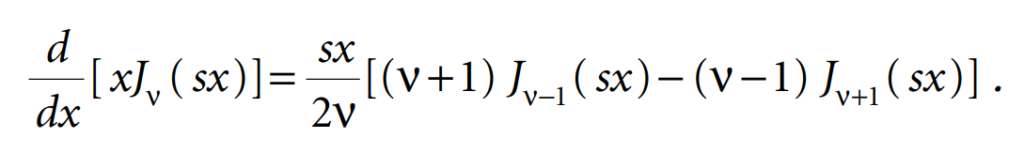
- Derivatives. Let
Proof,
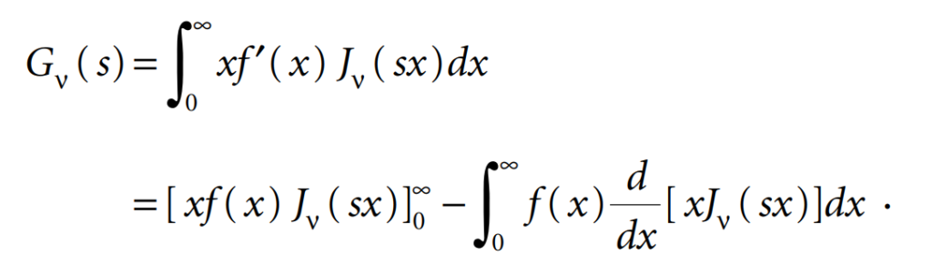
In general, the expression between the brackets is zero, and
2. The Hankel transform of the Bessel differential operator. The Bessel differential operator
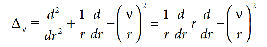
is derived from the Laplacian operator
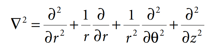
after separation of variables in cylindrical coordinates (r, θ, z).
Let ƒ(r) be an arbitrary function with the property that ƒ(r→∞) = 0. Then
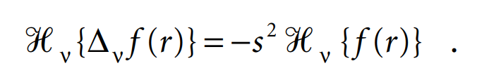
This result shows that the Hankel transform may be a useful tool in solving problems with cylindrical symmetry and involving the Laplacian operator.